Table of Contents
In this tutorial you will learn how to run a two-dimensional Reynolds-Averaged-Navier-Stokes simulation (2D RANS) of the (unactuated) flat plate using the 2D structured grid created in the previous tutorial. For more details about the numerical methods, please refer to the following sections on the structured grid and the structured finite volume solver.
Theory
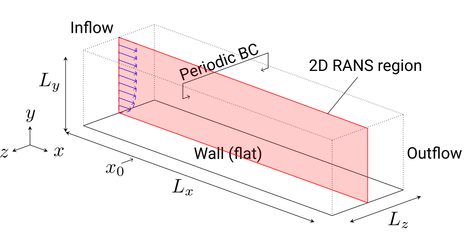
The figure below provides an overview of the unactuated flat plate used for the 2D RANS. More information about the numerical setup and methods can be found in this paper [Albers2020].
Tutorial
This tutorial is split into two parts, one for runnning the 2D RANS and one for post-processing the simulations results with focus on the skin friction coefficient.
Run the 2D RANS
Download and unzip this tutorial here and change the directory to the 2D RANS folder
2_rans:cd 2_rans
Create symbolic links to the compiled MAIA executable (if not already, please refer to the setup tutorial), the 2D RANS grid created in the previous tutorial and to the Python files which are needed to plot/analyze the convergence and to reset/clear the tutorial for the next test run. The last mentioned files are located one level up in the
toolsfolder:
ln -s maiaDirectory/Solver/src/maia maialn -s ../1_grid/grid_rans.hdf5 grid_rans.hdf5ln -s ../tools/rans/plot_rans_convergence.py plot_rans_convergence.pyln -s ../tools/rans/clear_rans.py clear_rans.pyTest if MAIA is correctly linked by opening MAIA's help:
maia -h
Open and have a look at the
properties_run_rans.tomlfile, which contains the settings used for running the 2D RANS with the structured grid:
Porperty Explanation Ma Mach number Re momentum thickness based Reynolds number \( \mathrm{Re}_{\theta} = u_{\infty} \theta / \nu \) at \( x_0 \) gridInputFileName Structured grid file used for the 2D RANS, like "./grid_rans.hdf5"solutionOutput Output directory for solution files, like "./out/"restartVariablesFileName Name of the restart file to restart/continue the simulation, like "./restart_rans.hdf5"timeSteps Final number of timesteps to simulate, e.g., 20000solutionInterval Output interval in timesteps resp. interval after which the solutions are saved every time, e.g., 10000rescalingBLT Rescaling factor concerning the boundary layer theory, delta99 at the inflow fullRANS Boolean for using RANS, i.e., trueransMethod RANS method, e.g., "RANS_SA_DV"for the Spalart-Allmaras turbulence model???solvertype.0 Solver part of MAIA, e.g., "MAIA_STRUCTURED"for the structured finite volume solver
Run the 2D RANS in sequence with the following command:
maia properties_run_rans.tomlTip: Allocate some computational resources for running the 2D RANS. By utilizing OpenMPI you can run the simulation in parallel using
noCoresprocessors:mpirun -np noCores maia properties_run_rans.toml- Note
- With a 12 core node (which processors???) the simulation should take about 5 minutes. Check that!!!
The print message on the console should look like this:
Global MPI informationMPI Info: nkeys = 1MPI Info: [0] key = nc_header_align_size, value = 10240_____ ______ ________ ___ ____________|\ _ \ _ \ |\ __ \ |\ \ |\ __ \ ______\ \ \\\__\ \ \\ \ \|\ \\ \ \\ \ \|\ \ ______\ \ \\|__| \ \\ \ __ \\ \ \\ \ __ \ ______\ \ \ \ \ \\ \ \ \ \\ \ \\ \ \ \ \ ______\ \__\ \ \__\\ \__\ \__\\ \__\\ \__\ \__\ ______\|__| \|__| \|__|\|__| \|__| \|__|\|__| ____Start time: 2023-02-02 13:57:31Number of ranks: 12Number of OMP threads: 36Host (of rank 0): aia315Working directory: maiaTutorialDirectory/2_ransUser: YourNameExecutable: maiaCommand line args: maia properties_run_rans.tomlm_noSolvers: 1=== MAIA RUN LOOP ====== MAIA RUN DURATION: Create geometries | min: 6.9141e-06 s | avg: 9.4970e-06 s | max: 1.2875e-05 s |=== Create grid...=== Create structured grid...=== done.=== MAIA RUN DURATION: Create grid | min: 3.6001e-05 s | avg: 4.4008e-05 s | max: 5.1022e-05 s |FV-MB is offFV-LS is offLB is offLB LS is offLS SOLVER is offCOMBUSTION is offDG is offLS-RANS is off=== Create solvers...=== Create structured solver...Initializing Structured Solver...Doing block decomposition...=== PARALLELIO FILE LIFETIME: ./grid_rans.hdf5 | 8.7371e-03 s |Doing block decomposition... SUCCESSFUL!=== PARALLELIO FILE LIFETIME: ./grid_rans.hdf5 | 2.3416e-02 s |=== PARALLELIO FILE LIFETIME: ./grid_rans.hdf5 | 1.6129e-03 s |=== PARALLELIO FILE LIFETIME: ./grid_rans.hdf5 | 7.7295e-04 s |Starting grid connection info search...Reading in all coordinates of all block facesoffset[1]=0 offset[0]=0size[1]=1 size[0]=55offset[1]=23 offset[0]=0size[1]=1 size[0]=55Loading periodic face coordinatesBuilding up connections for multiblock connection searchComputing periodic window displacementswe have evenSides 0 and we have oddSides 0 in BlockId 0we have evenSides 0 and we have oddSides 0 in BlockId 0...=== MAIA RUN DURATION: Full initialization | min: 1.8187e-01 s | avg: 1.8256e-01 s | max: 1.8283e-01 s |0 ThetaInflow 1.00631463 ThetaRecyclingStation 1.232240410 ThetaInflow 1.00480941 ThetaRecyclingStation 1.233690110 ThetaInflow 0.99865672 ThetaRecyclingStation 1.240805520 ThetaInflow 1.00309626 ThetaRecyclingStation 1.23554359...0 ThetaInflow 0.99898883 ThetaRecyclingStation 1.150953990 ThetaInflow 0.99897972 ThetaRecyclingStation 1.151497120 ThetaInflow 0.99898169 ThetaRecyclingStation 1.152013010 ThetaInflow 0.99897661 ThetaRecyclingStation 1.152513650 ThetaInflow 0.99897937 ThetaRecyclingStation 1.152994820 ThetaInflow 0.99898358 ThetaRecyclingStation 1.153453050 ThetaInflow 0.99898784 ThetaRecyclingStation 1.153893350 ThetaInflow 0.99900187 ThetaRecyclingStation 1.154308120 ThetaInflow 0.99902361 ThetaRecyclingStation 1.15469164=== PARALLELIO FILE LIFETIME: ./out/auxData20000.hdf5 | 1.4262e-02 s |=== PARALLELIO FILE LIFETIME: ./out/20000.hdf5 | 2.1094e-02 s |******************************* MEMORY STATISTICS ************************************ Comment: After run loop - #ranks: 12***** Location: void MAIAApplication::run() [with int nDim = 2] (maiaDirectory/Solver/src/application.cpp:1137)********** Average memory usage: physical = 27.7067 MB; allocation = 77.0055 MB***** Minimun memory usage: physical = 26.8281 MB; allocation = 74.9492 MB***** Maximum memory usage: physical = 34.2188 MB; allocation = 99.0977 MB***** Maximum diff in memory usage: physical = 34.2188 MB; allocation = 99.0977 MB***** Total physical memory usage (RAM): 0.324688 GB***** Diff total physical memory usage (RAM): 0.324688 GB***** Total allocation size (Virtual Memory): 0.902409 GB***** Diff total allocation size (Virtual Memory): 0.902409 GB********** Maximum stack memory: 136 KB; stack limit 8192 KB********** Minimum available memory per node (meminfo): 196.453 GB***** Minimum free memory per node (RAM): 63.5602 GB******************************* MEMORY STATISTICS *******************************Running the simulation results in the following files:
File(s) Explanation 2_rans/out/SomeTimestep.hdf5 Solution files for predefined timestep intervals, like 10000.hdf52_rans/out/auxData20000.hdf5 Auxiliary solution files for the final timestep. Purpose??? 2_rans/maia_log Log file containing information of how the simulation has run 2_rans/Residual Residuals of the simulation for every timestep 2_rans/theta_inflow.dat Momentum-based boundary layer thickness \( \delta_2 = \theta \) at \( x_0 = 0 \) for every timestep
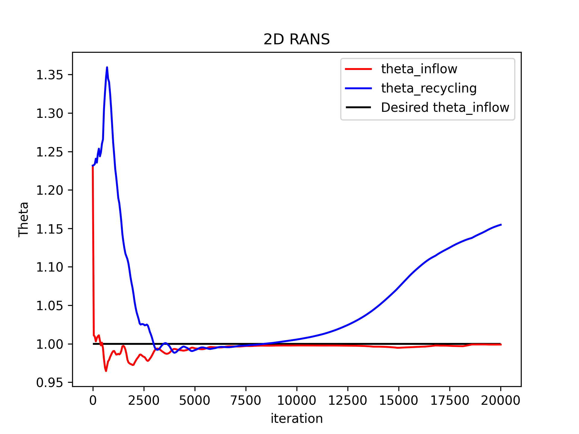
Check if the solution is converged and if \( \delta_2 (x_0 = 0) = \theta (x_0 = 0) = 1 \), i.e.,
ThetaInflow = d2(x=0) = 1:python3 plot_rans_convergence.pyThe momentum-based boundary layer thickness \( \delta_2 (x_0 = 0) = \theta (x_0 = 0) \) at the inflow \( x_0 = 0 \) against the number of timesteps should look like this:
The residuals against the number of timesteps should look like this:
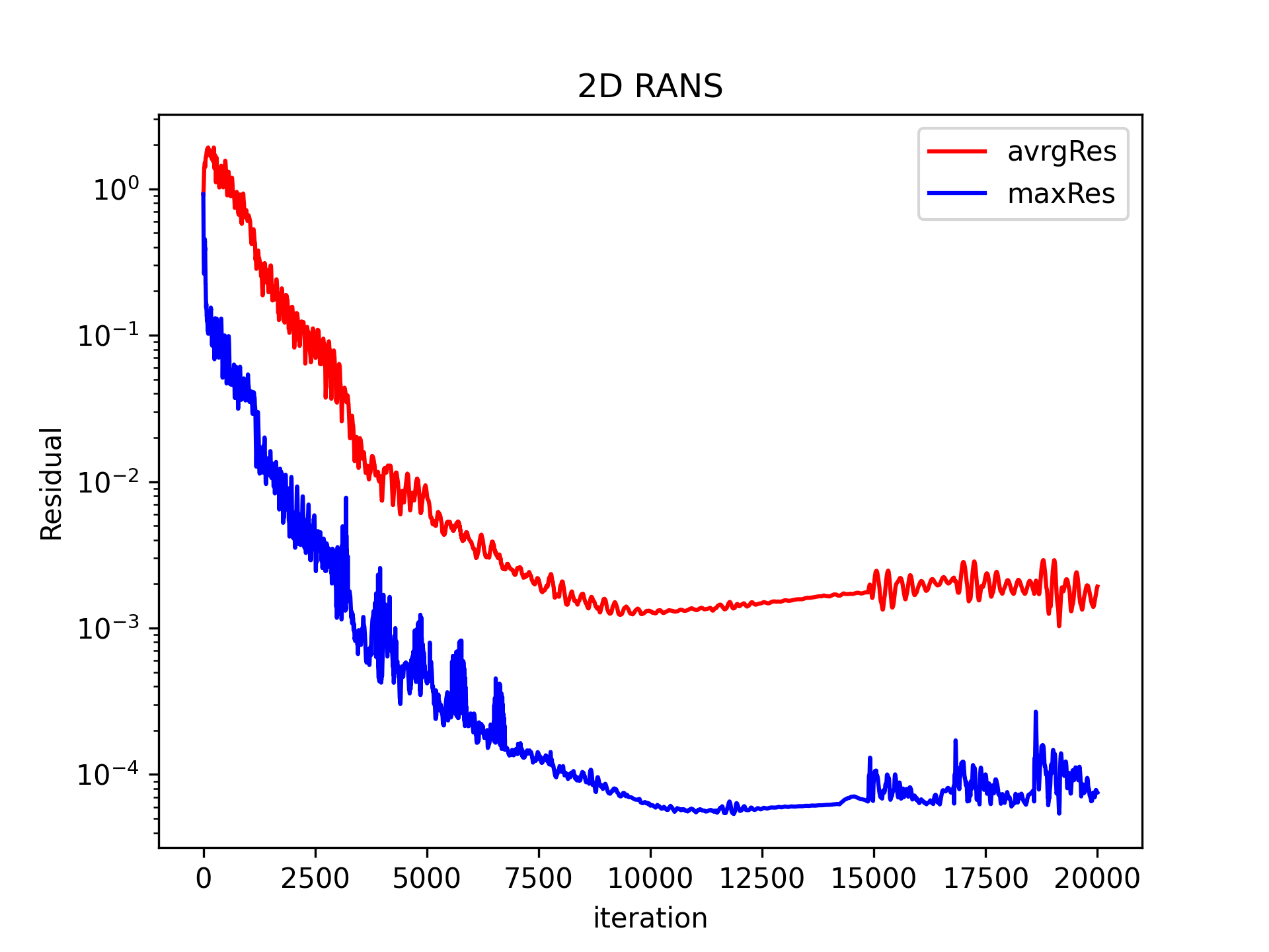
If not converged rerun/continue the RANS with a larger number of timesteps in
properties_run_rans.toml:Rerun the RANS:
python3 clear_rans.pyOpen
properties_run_rans.toml, increase the number of timesteps denoted as the porpertytimeSteps, save it and jump to step 4.Restart/Continue from the current RANS: How to continue??? Do we even need to show that??? Currently no restart file created/used!
If not d2(x=0)=1 adjust
rescalingBLTparameter inproperties_run_rans.tomland rerun the 2D RANS untilThetaInflow = d2(x=0) = 1. This condition must be meet to achieve the desired and predefined Reynolds number. The following rule of thumb can be used to select the new rescaling factor based on the previous/old convergedThetaInflow:Condition to meet:
1 = ThetaInflow_converged_new = ThetaInflow_converged_old / rescalingBLT_old * rescalingBLT_newResulting rule of thumb to select the new rescaling factor
rescalingBLT_new:rescalingBLT_new = rescalingBLT_old / ThetaInflow_converged_oldRerun the RANS:
python3 clear_rans.pyOpen
properties_run_rans.toml, change the boundary layer rescaling factor denoted as the porpertyrescalingBLTto the value of the newly computedrescalingBLT_new, save it and jump to step 4.
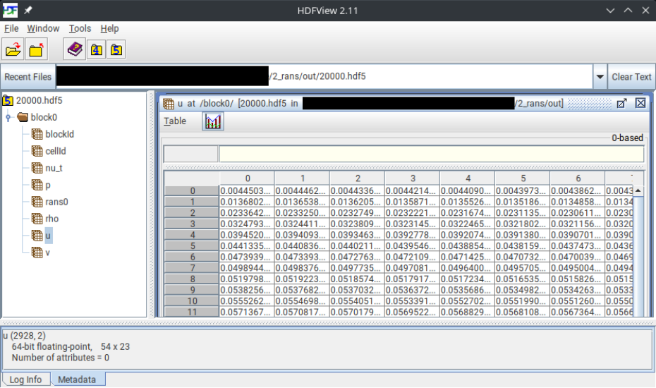
Check plausibility of the flow:
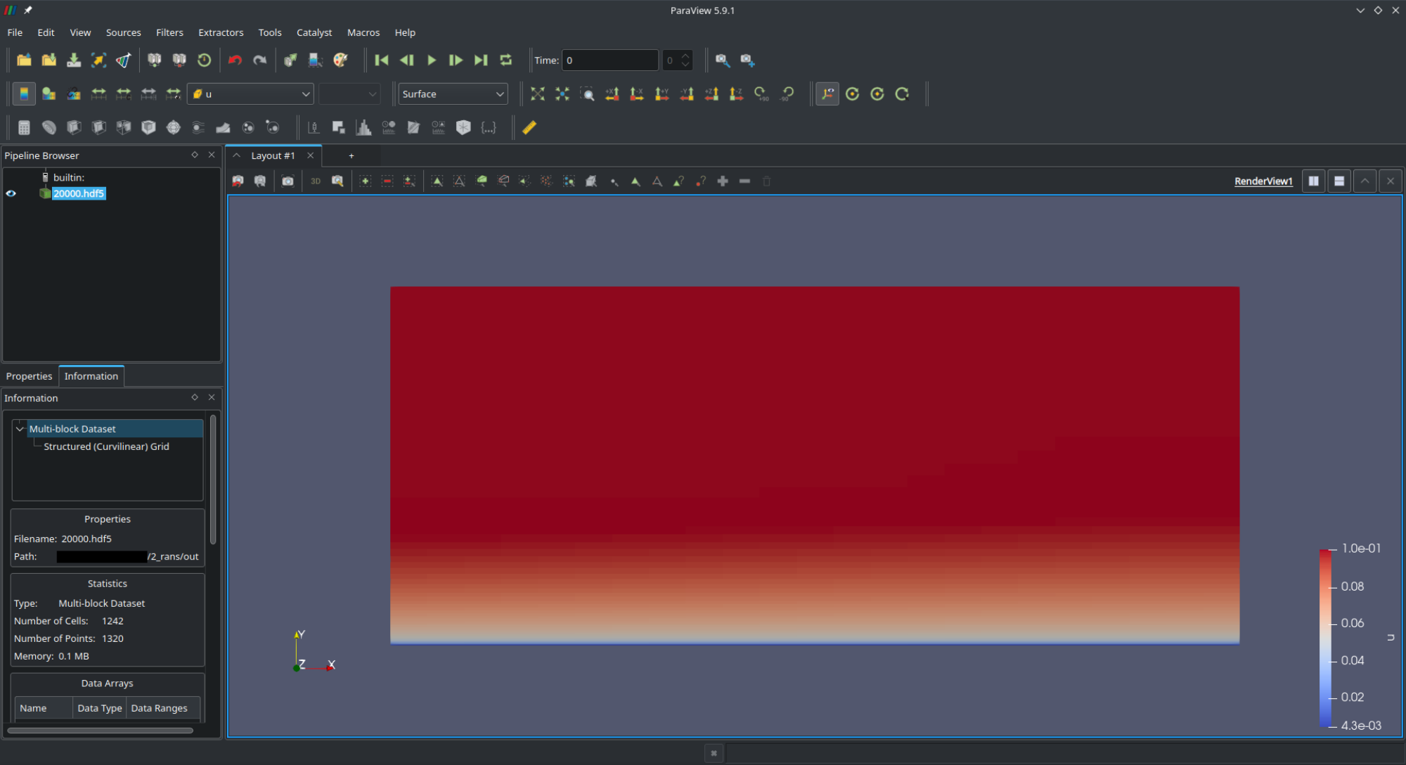
Check the last hdf5-solution file
LastTimestep.hdf5, e.g.,20000.hdf5, with HDFViewcd outhdfview LastTimestep.hdf5The hdf5-solution file should look like this:
or with ParaView
cd outparav LastTimestep.hdf5The hdf5-solution file should look like this when using the \( u \) velocity component and the visualization as a surface:
Post-process the 2D RANS
Download and unzip
bltools.pyin thetoolsfolder: Currently,bltools.pyand the corresponding post-processing scripts are located intools. Where to get the newest version ofbltools.py: https://git.rwth-aachen.de/aia/MAIA/tools/-/tree/master/postprocessing/structured/blpp
Change the directory to the post-processing folder
postand create symbolic links to the post-processing scripts in thetoolsfolder. Currently thedatais not created automatically, therefore it has to be created by the user withmkdir data:cd ..cd postln -s ../../tools/bltools.py bltools.pyln -s ../../tools/rans/plot_cf_rans.py plot_cf_rans.pyln -s ../../tools/rans/plot_delta_xyz_plus.py plot_delta_xyz_plus.pymkdir data
Run the post-processing evaluation file
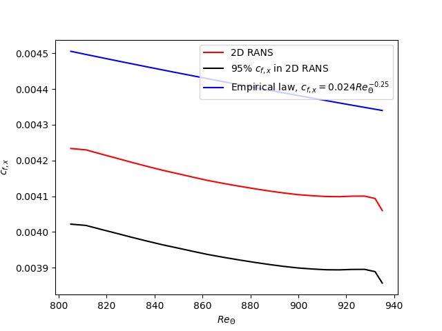
eval_rans.py, for example to calculate the streamwise skin friction coefficient \( c_{f,x} = \frac{ 2 \tau_{\mathrm{wall}} }{ \rho_{\infty} v^2_{\infty} }\) (local drag coefficient):python3 eval_rans.pyThe print message on the console should look like this:
NumPy version: 1.17.3#################################### PARAMETERS ####################################MA: 0.1RE: 800.0 <- for the grid a different Reynolds number was used. Adjust it!T8: 0.998003992015968U8: 0.0999001497504367RHO8: 0.9950174476440005MUE8: 0.9984267285780992RE0: 8035.434224461798P8: 0.7093081320530371Base folder: ../Grid folder: ../Solutionfolder: ../out/Output folder: ./data/Output name: referenceCase type is refLoading grid...Dimensions in grid file: 2noPointsJ: 55 noPointsI: 24Loading grid... FINISHED!Computing cell centers...Computing cell centers... FINISHED!############################Loading 2D postprocessing variables...no_cells[0]: 54 no_cells[1]: 23Loading 2D postprocessing variables... FINISHED!no_cells[J]: 54 no_cells[I]: 23Computing wall properties...Computing wall properties... FINISHED!Computing wall shear stress...Computing wall shear stress... FINISHED!Begin searching streamwise position...current J: 0 current I: 1grid.no_cells[0]: -1 grid.no_cells[1]: 54 grid.no_cells[2]: 23Attention!! Grid coordinate is still with : K 0 J 1 I 2[3, 7]Successfully find streamwise positions with ipos... FINISHED!Computing velocity distribution...Computing velocity distribution... FINISHED!The resulting files are:
File(s) Explanation 2_rans/post/data/bl_reference.dat Boundary layer reference data 2_rans/post/data/profile_reference_iposNum.dat Post-processing results at certain i-positions - Note
- In principle the
bl_reference.npzcontains the same information as thebl_reference.dat, but consisting of multiple zippednpy-files tailored to the use of Python.
Visualize the drag coefficient and check if the 2D RANS results are porper to use for the next tutorial dealing with the Synthetic Turbulence Generation (STG):
python3 plot_cf_rans.pyWhat means proper (comparison with the empirical law) and why 95% of the empirical law? And where does the empirical formula come from?
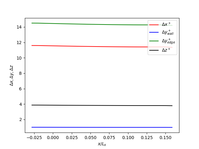
Check the evolution of the grid resolution along the streamwise direction:
python3 plot_delta_xyz_plus.pyThe resulting plot should look like this:
- Note
- The grid resolution at the wall is much finer than the resolution distant from the wall, since we want to resolve the turbulent flow at the wall.
- Todo:
- Adjust units displayed by the plot method.
TODOs
- Rerun the simulation with re=1000 instead of re=800, and update the printed messages on the console and the images!
- Change the big theta \( \Theta \) to the small one \( \theta \) in the plots
References
- Albers, M., Meysonnat, P. S., Fernex, D., Semaan, R., Noack, B. R., & Schröder, W. (2020). Drag reduction and energy saving by spanwise traveling transversal surface waves for flat plate flow. Flow, Turbulence and Combustion, 105(1), 125-157. https://link.springer.com/article/10.1007/s10494-020-00110-8.